Andrew Ng

Introduction

Machine Learning definition

a computer program is said to learn from experience E with respect to some task T and some performance measure P, if its performance on T, as measured by P, improves with experience E

Tom Mitchell (1998)

下象棋：

(T) 任务：下象棋
(E) 经验: 下几万遍象棋的累积
(P) 性能指标：下一盘棋的成功概率

标记垃圾邮件：

T: 标记垃圾邮件的行为
E：观察你标记垃圾行为的历史
P：正确标记垃圾邮件的比例

Machine Learning algorithms：

Supervised learning
Unsupervised learning
Reinforcement learning
recommender systems

Supervised Learning

right answers given，the task is to produce more these right answers
In supervised learning, we are given a data set and already know what our correct output should look like, having the idea that there is a relationship between the input and the output.

Regression Problem

Predict continuous valued output, meaning that we are trying to map input variables to some continuous function.

e.g. Given data about the size of houses on the real estate market, try to predict their price. Price as a function of size is a continuous output e.g. Given a picture of a person, we have to predict their age on the basis of the given picture

Classification Problem

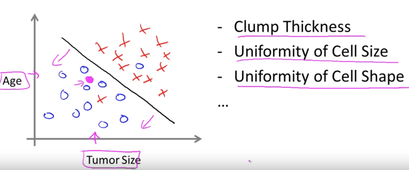
we are trying to map input variables into discrete categories. 根据给定的数据集，判断一个数据应该归属于哪个类别，

e.g. from the last house price example, we making our output about whether the house "sells for more or less than the asking price. e.g. Given a patient with a tumor, we have to predict whether the tumor is malignant or benign. (图中展示了年龄和肿瘤大小，实际中可能有更多，甚至无限多的指标)

Unsupervised Learning

Unsupervised learning allows us to approach problems with little or no idea what our results should look like. We can derive structure from data where we don't necessarily know the effect of the variables.

We can derive this structure by clustering the data based on relationships among the variables in the data.

With unsupervised learning there is no feedback based on the prediction results.

Clustering

e.g. Take a collection of 1,000,000 different genes, and find a way to automatically group these genes into groups that are somehow similar or related by different variables, such as lifespan, location, roles, and so on.

Non-clustering

e.g. The "Cocktail Party Algorithm", allows you to find structure in a chaotic environment. (i.e. identifying individual voices and music from a mesh of sounds at a cocktail party).

One variable Linear regression

Model representation and Cost function

Hypothesis: $h_\theta(x) = \theta_0 + \theta_1x$ Parameters: $\theta_0, \theta_1$ Cost Function: $J(\theta_0, \theta_1) = \frac{1}{2m}\sum_{i=1}^m(\hat{y}_i-y_i)^2 = \frac{1}{2m}\sum_{i=1}^m(h_\theta(x_i)-y_i)^2$ Goal: $\underset{\theta_0, \theta_1}{\rm minimize}J(\theta_0, \theta_1)$

m: the size of traning dataset，比如889条
1/m: 是为了求平均数
1/2: 是为了在二项式求导时能消掉

This function is otherwise called the Squared error function, or Mean squared error. (最小二乘法)

Gradient descent algorithm

即梯度下降法

repeat until convergence {
$\quad\theta_j := \theta_j - \alpha\frac{\partial}{\partial\theta_j}J(\theta_0, \theta_1)\quad(\rm simultaneously\ update\ j=0\ and\ j=1)$ }

the derivative of a scalar valued multi-variable function always means the direction of the steepest ascent, so if we want to go desent direction, we minus the derivative.

plug in the $h_\theta(x)$ and $J(\theta_0, \theta_1)$ , we got

\begin{cases} \theta_0 := \theta_0-\alpha\frac{\partial}{\partial\theta_0}\frac{1}{2m}\sum_{i=1}^m(h_\theta(x_i)-y_i)^2 \\ \theta_1 := \theta_1-\alpha\frac{\partial}{\partial\theta_1}\frac{1}{2m}\sum_{i=1}^m(h_\theta(x_i)-y_i)^2 \end{cases} \Rightarrow \begin{cases} \theta_0 := \theta_0-\alpha\frac{1}{m}\sum_{i=1}^m(h_\theta(x_i)-y_i) \\ \theta_1 := \theta_1-\alpha\frac{1}{m}\sum_{i=1}^m(h_\theta(x_i)-y_i) \cdot x_i \end{cases}

the partial derivative of $\theta_1$ use chain rule apparently.

the cost function for linear regression is always going to be a bow shaped function called Convex function, so this function doesn't have any local uptimum but one global uptimum.

Batch Gradient Descent

we also call this algorithm Batch Gradient Descent, batch means each step of gradient descent uses all the training examples.

Multivariate Linear Regression

Multiple Features

如果多了几个参数：

size	rooms	flats	ages	price
127.3	8	2	15	235,72
89.5	3	1	8	17,345
...

Linear regression with multiple variables is also known as "multivariate linear regression". The multivariable form of the hypothesis function accommodating these multiple features is as follows:

$h_\theta(x)=\theta_0+\theta_1x_1+\theta_2x_2+\theta_3x_3+\cdots+\theta_nx_n$

为了写成矩阵形式，我们补一个 $x_0=1$ ，则 $h_\theta(x)=[\theta_0\ \theta_1\ \cdots\ \theta_n]\cdot \begin{bmatrix} x_0\\ x_1\\ \vdots x_n \end{bmatrix} = \theta^T \cdot x$ while the cost function as: $J(\theta) = \frac{1}{2m}\sum_{i=1}^m(h_\theta(x^{(i)})-y^{(i)})^2$

这里用了 $x^{(i)}$ 而不是 $x_i$ ，是为了更严谨，右上角表示第几组训练数据，右下角用来表示第几个feature, 即 $x^{(3)}_4$

the gradient descent: Repeat { $\quad\theta_j:=\theta_j-\alpha\frac{\partial}{\partial\theta_j}J(\theta)\;(\small\rm simultaneously\ update\ for\ every\ j=0,\dots,n)$ } plug the $J(\theta)$ in:

$\theta_j:=\theta_j-\alpha\frac{1}{m}\sum_{i=1}^{m}(h_\theta(x^{(i)})-y^{(i)})\cdot x^{(i)}_j$

其中 $x^{(i)}_j$ 就是 $\theta_j \cdot x^{(i)}_j$ 对 $\theta_j$ 求的导数。

Feature Scaling

Get every feature into approximately a $-1\leq x_i \leq 1$ range (to make sure features are on a similar scale).

Mean Normalization

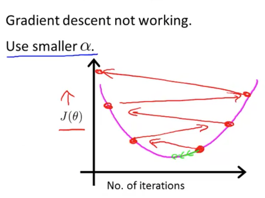
Replace $x_i$ with $x_i-u_i$ to make features have approximately zero mean (Do not apply to $x_0$ , because it's always be 1): $x_i=\frac{x_i-u_i}{s_i}$ $u_i$ : the average of $x_i$ in training set $s_i$ : the range of $x_i$ , aka: max-min, OR, the standard deviation 如果size平均在1000feets左右，数据集的跨度在2000，那么可以设 $x_1=\frac{size-1000}{2000}$ ，这样 $x_i$ 就落在了 $-0.5\leq x_i \leq 0.5$

debuging Learing rate

debuging making sure gradient descent is working correctly. $J(\theta)$ should decrease after every iteration (for a sufficiently small $\alpha$ ). 比如你发现曲线向上了，可能是选择了不恰当（过大）的learning rate（ $\alpha$ ），而如果收敛得太慢了，那可能是选择了一个太小的learning rate。

Features and polynomial regression

We can improve our features and the form of our hypothesis function in a couple different ways. We can combine multiple features into one. For example, we can combine $x_1$ and $x_2$ into a new feature $x_3$ by taking $x_1\cdot x_2$ ,(比如房间的进深和宽度变成房子的面积)

Our hypothesis function need not be linear (a straight line) if that does not fit the data well. We can change the behavior or curve of our hypothesis function by making it a quadratic, cubic or square root function (or any other form). (会形成抛物线 $-x^2$ ，上升曲线( $x^3, \sqrt2$ )等等)

For example, if our hypothesis function is $h_\theta(x)=\theta_0+\theta_1x_1$ then we can create additional features based on $x_1$ , to get the quadratic function $h_\theta(x)=\theta_0+\theta_1x_1+\theta_2x_1^2$ or qubic function $h_\theta(x)=\theta_0+\theta_1x_1+\theta_2x_1^2+\theta_3x_1^3$

we just need to set $x_2=x^2_1$ and $x_3=x_1^3$ and, the range will be significantly change, you should right normalization your data (feature scaling).

Computing Parameters Analytically

Normal equations method

除了梯度下降，我们还可以用Normal equation来求极值， a Method to solve for $\theta$ analytically。

简化到一个普通的抛物线，我们知道其极值显然就是其导数为0的地方，所以我们可以用求 $\frac{d}{d\theta}h_\theta(x)=0$ ，在多项式里，我们补齐 $x_0=1$ 的一列为参数矩阵 $X$ ， $\theta$ 取如下值是有最小值： $\theta=(X^TX)^{-1}X^Ty$

and There's no need to do feature scaling with the normal equation

Gradient Descent	Normal Equation
Need to choose alpha	No need to choose alpha
Needs many iterations	No need to iterate
$O(kn^2)$	$O(n^3)$ need to calculate inverse of X
Works well when n is large	Slow if n is very large

Noraml Equation Noninvertibility

in octave, we can use pinv rather inv. the pinv function will give you a value of $\theta$ even if $X^TX$ is not invertible. the p means pseudo.

It's common causes by:

Redundant features, where two features are very closely related (i.e. they are linearly dependent)
Too many features (e.g. m ≤ n). In this case, delete some features or use "regularization" (to be explained in a later lesson).

Logistic Regression

Classfication and Representation

For now, we will focus on the binary classification problem in which y can take on only two values, 0 and 1 $\Rightarrow \ y\in\{0,1\}$ .

To attempt classification, one method is to use linear regression and map all predictions greater than 0.5 as a 1 and all less than 0.5 as a 0. However, this method doesn't work well because classification is not actually a linear function.

比如把0.8映射成1是合理的，但800呢？ $h_\theta$ 可能远大于1或远小于0，在明知目标非0即1的情况下，这是不合理的，由此引入了 $0 \leq h_\theta \leq 1$ 的Logistic Regression（其实是一个classification algorithm)。

Hypothesis Representation

线性回归的( $\theta^Tx$ )并不能很好地用来表示classification problem，但我们可以基于其来选择一个函数(g)，让它的输出值在(0,1)之间，这个函数叫Sigmoid Function或Logistic Function:

$h_\theta(x) = g(\theta^Tx)$
$z = \theta^Tx$
$g(z) = \frac{1}{1+e^{-z}}$

Sigmoid就叫S型函数，因为它的图像是这样的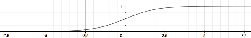： The function g(z), shown here, maps any real number to the (0, 1) interval, making it useful for transforming an arbitrary-valued function into a function better suited for classification.

正确理解Sigmoid函数，它表示的是在给定的（基于 $\theta$ 参数的）x的值的情况下，输出为1的概率。

$h_\theta(x) = P(y = 1\ |\ x;\theta)$

显然，y=1与y=0的概率是互补的。

Decision boundary

从上节的函数图像可知， $z=0$ 就是0.5的分界点，而 $z = \theta^Tx$ 就是 $g(z)$ 的入参： $\begin{cases} h_\theta(x) \geq 0.5 \rightarrow y=1 \\ h_\theta(x) \lt 0.5 \rightarrow y=0 \end{cases} \Rightarrow g(z) \geq 0.5\ when\ z \geq 0 \Rightarrow \theta^Tx \geq 0$

同时， $g(z) = \frac{1}{1+e^{-z}}$ 得知z趋近无穷大，g(x)越趋近1，反之越趋近0，意味着越大的z值越倾向于得到y = 1的结论。

The decision boundary is the line that separates the area where y = 0 and where y = 1. It is created by our hypothesis function. 基本上，它就是由 $\theta^Tx=0$ 确立的。

记住， $\theta_i$ 的值都是估计值，正确地选择（或不同地选择） $\theta$ 会导致不同的dicision boundary，选择也是充满技巧的。

例: 对于 $h_\theta(x) = g(\theta_0 + \theta_1x_1 + \theta_2x_2)$ ，如果取: $\begin{aligned} & \theta = \begin{bmatrix}5\\-1\\0\end{bmatrix} \\ & y = 1\ {\color{red}if}\ 5 + (-1)x_1 + 0x_2 \geq 0 \\ & \Rightarrow x_1 \leq 5 \end{aligned}$

而选 $[-3, 1, 1]^T$ ，则有 $x_1+x_2=3$

这将是两条不同的直线，即不同的dicision boundary

更复杂的例子： $h_\theta(x) = g(\theta_0+\theta_1x_1+\theta_2x_2+\theta_3x_1^2+\theta_4x_2^2)$ ，巧妙地设 $\theta = [-1, 0, 0, 1, 1]$ ，将会得到 $x_1^2 + x_2^2 = 1$ ，这就是一个圆嘛。

Again, the decision boundary is a property, not of the traning set, but of the hypothesis under the parameters. (不同的 $\theta$ 组合，给出不同的decision boundary)

Cost function

$J(\theta)=\frac{1}{m}\sum_{i=1}^{m}Cost(h_\theta x^{(i)},y^{(i)})$

$Cost(h_\theta(x), y) =\begin{cases} -log(h_\theta(x)) & if\ y=1 \\ -log(1-h_\theta(x)) & if\ y=0 \end{cases}$

引入log是为了形成凸函数（convex），-log(z)与-log(1-z)的函数图形分别如下，取(0,1)部分：

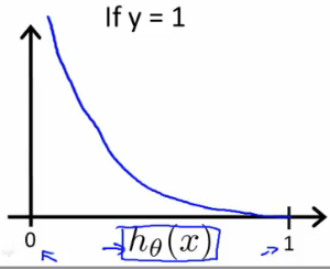
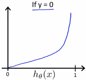
注意： $z=h_\theta(x)$

从图像分析，我们能得到如下结论：

当y = 0时，如果 $h_\theta x = 0$ （语义为y=1的概率为0），cost function也为0，即预测很精确，语义上也是相同的，y=0时y=1的概率当然是0
当y = 0时，如果 $h_\theta x = 1$ （语义为y=1的概率为100%），cost function也为无穷大，即误差无限大，语义上，y=0当然不能与y=1并存

Simplified cost function and gradient descent

Simplify Cost function

上节两个等式可以简化为：

$Cost(h_\theta(x),y) = -ylog(h_\theta(x)) - (1-y)log((1-h_\theta(x^{(i)})))$

很好理解，y只能为0或1，y和(1-y)必有一个是0，所以：

$\begin{aligned} J(\theta) & = \frac{1}{m}\sum_{i=1}^mCost(h_\theta(x),y) \\ & = -\frac{1}{m}\sum_{i=1}^m[ y^{(i)}log(h_\theta(x^{(i)})) + (1-y^{(i)})log(1-h_\theta(x^{(i)})) ]\end{aligned}$

from the principle of maximum likelihood estimation(最大似然估计)

for $\underset{m}{min}J(\theta)$ get the $\theta$ ， the output: $h_\theta(x) = \frac{1}{1+e^{-\theta^Tx}}$ ，意思是给定x能得到 $p(y=1 | x;\theta)$ ，即y=1的概率，即完成了clasification。

A vectorized implementation is:

$h=g(X\theta)$

$J(\theta) = -\frac{1}{m}\cdot(-y^Tlog(h)-(1-y)^Tlog(1-h))$ （交叉熵损失Binary Cross Entropy Loss）

Gradient Descent

$\theta_j:=\theta_j - \alpha\frac{\partial}{\partial\theta_j}J(\theta) \Rightarrow \theta_j:=\theta_j - \frac{\alpha}{m}\sum_{i=i}^{m}(h_\theta(x^{(i)}) - y^{(i)})x_j^{(i)}$

Looks identical to linear regression

for linear regression, $h_\theta(x) = \theta^Tx$
for logistical regression, $h_\theta(x) = \frac{1}{1+e^{-\theta^Tx}}$
线性回归里 $\theta^Tx$ 与y相减就是损失函数，逻辑回归里， $\theta^Tx$ 要代入到上述log函数里才是损失函数!!!

这里为什么损失函数分明不是 $h_\theta(x) - y$ 求导后仍然变成这个形式了呢？下面截图有求导过程，可见它只是恰好是这个形态，但是千万不要认为这才是推导依据，这就是数学之美吧。

求导过程：

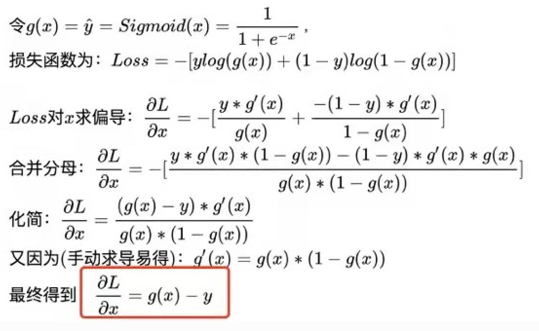
以后再自己试自己按行求导再求和，对于矩阵，还是用矩阵求导的链式法则： $z = f(Y),\ Y = AX+B \Rightarrow \frac{\partial z}{\partial X} = A^T\frac{\partial z}{\partial Y}$ 即先对四则运算进行求导，然后再根据矩阵在x左边还是右边来左乘或右乘 $A^T$ reference

所以： $\theta := \theta - \frac{\alpha}{m}X^T(g(X\theta) - \vec{y})$

解释：

cost function是那一串log相减，最外层求导后就是 $h(x)-y$

而 $h(x) = g(X\theta)$ ，应用链式法，内层就是 $X\theta$ 对 $\theta$ 继续求导，结果是把 $X^T$ 乘到左边去

直接用emoji字符把𝜃写到方法名里去，直接还原公式，如果有对老师代码与公式的对照产生疑惑的，看看有没有更直观

Advanced optimization

Conjugate gradient（共轭梯度）, BFGS（局部优化法, Broyden Fletcher Goldfarb Shann）, and L-BFGS（有限内存局部优化法） are more sophisticated, faster ways to optimize θ that can be used instead of gradient descent. 这些算法有一个智能的内部循环，称为线性搜索(line search)算法，它可以自动尝试不同的学习速率。只需要给这些算法提供计算导数项和代价函数的方法，就可以返回结果。适用于大型机器学习问题。

We first need to provide a function that evaluates the following two functions for a given input value θ:

$\begin{aligned} &J(\theta) \\ &\frac{\partial}{\partial\theta_j}J(\theta) \end{aligned}$

then wirte a single function that returns both of these:

function [jVal, gradient] = costFunction(theta)
  jVal = [...code to compute J(theta)...];
  gradient = [...code to compute derivative of J(theta)...];
end

Then we can use octave's fminunc() optimization algorithm along with the optimset() function that creates an object containing the options we want to send to "fminunc()".

options = optimset('GradObj', 'on', 'MaxIter', 100);
initialTheta = zeros(2,1);
   [optTheta, functionVal, exitFlag] = fminunc(@costFunction, initialTheta, options);

Multi-class classfication: One-vs-all

One-vs-all -> One-vs-rest，每一次把感兴趣的指标设为1，其它分类为0，其它指标亦然，也就是说对每一次分类，都是一次binary的分类。

$h_\theta^{(i)}(x) = P(y=i\ |\ x;\theta)\quad(i=1,2,3...)$ 这样就得到了i为1，2，3等时的概率，概率最大的即为最接近的hypothesis。

Regularization

The problem of overfitting

如果样本离回归曲线（或直线）偏差较大，我们称之为underfitting，而如果回归曲线高度贴合每一个样本数据，导致曲线歪歪扭扭，这样过度迎合了样本数据，甚至包括特例，反而非常不利于预测未知的数据，这种情况就是overfitting，过度拟合了，它的缺点就不够generalize well。

如果我们的feature过多，而训练样本量又非常小，overfitting就非常容易发生。

Options:

Reduce number of features
- Manually select which features to keep.
- Model selection algorithm (later in course).
Regularization
- Keep all the features, but reduce magnitude/values of parameters $\theta_j$ .
- Works well when we have a lot of features, each of which contributes a bit to predicting $y$ .

Regularization

Cost function

Samll values for parameters $\theta_0, \theta_1, \dots, \theta_n$

"Simpler" hypothesis
Less prone to overfitting

Housing:

Features: $x1, x2, \dots, x100$
Parameters: $\theta_0, \theta_1, \dots, \theta_100$

J(\theta) = \frac{1}{2m} \left[ \sum_{i=1}^m(h_\theta(x^{(i)}) - y^{(i)})^2 \overbrace{\red{+ \lambda\sum_{j=1}^n\theta_j^2}}^{\tt \small regulation\ term} \right]

and $\lambda$ here is regularization parameter, It determines how much the costs of our theta parameters are inflated.

We've added two extra terms at the end to inflate the cost $\theta_j(1,n)$ , Now, in order for the cost function to get close to zero, we will have to reduce the values of $\theta_j$ s to near zero. 一般这些都发生在高阶的参数上，比如 $\theta_3x^3,\ \theta_4x^4$ ，这些值将会变得非常小，表现在函数曲线上，将会大大减小曲线的波动。

Regularized linear regression

我们不对 $\theta_0$ 做penalize，这样更新函数就变成了：

\begin{aligned} &\theta_0 := \theta_0 - \alpha\frac{1}{m}\sum_{i=1}^m(h_\theta(x^{(i)}) - y^{(i)})x_0^{(i)} \\ &\theta_j := \theta_j - \alpha\left[ \left( \frac{1}{m}\sum_{i=1}^m(h_\theta(x^{(i)}) - y^{(i)})\cdot x_j^{(i)} \right) + \frac{\lambda}{2m}\theta_j^2 \right]\quad\quad j\in\{1,2,\dots,n\} \\ &\theta_j := \theta_j(1-\alpha\frac{1}{m}) - \alpha\frac{1}{m} \sum_{i=1}^m(h_\theta(x^{(i)}) - y^{(i)})x_j^{(i)} \end{aligned}

$1-\alpha\frac{1}{m} < 1$ ，可以直观地理解为它每轮都把 $\theta_j$ 减小了一定的值。

Normal Equation

\theta = (X^TX + \lambda \cdot L)^{-1}X^Ty

\tt where\ L = \begin{bmatrix} 0 &&&&\\ &1&&&\\ &&1&&\\ &&&\ddots&\\ &&&&1 \end{bmatrix}

Recall that if m < n, then $X^TX$ is non-invertible. However, when we add the term λ⋅L, then $X^TX+ λ⋅L$ becomes invertible.

Regularized Logistic Regression

Feature mapping

One way to fit the data better is to create more features from each data point. 比如之前的两个feature的例子，我们将它扩展到6次方：

\tt{mapped\ features}= \begin{bmatrix} 1\\x_1\\x_2\\x_1^2\\x_1x_2\\x_x^2\\x_1^3\\\vdots\\x_1x_2^5\\x_2^6 \end{bmatrix}

As a result of this mapping, our vector of two features has been transformed into a 28-dimensional vector. A logistic regression classifier trained on this higher-dimension feature vector will have a more complex decision boundary and will appear nonlinear when drawn in our 2-dimensional plot.

此时再画2D图时（表示decision boundary），就得用等高线了(contour)

J(\theta) =\frac{1}{m}\sum_{i=1}^m{\left[-y^{(i)} \log(h_{\theta}(x^{(i)}))-(1-y^{(i)}) \log(1-h_{\theta}(x^{(i)}))\right]} +\frac{\lambda}{2m}\sum_{j=1}^n{\theta_j^2}

求导时注意第1列x是补的1，也把 $\theta_0$ 给提取出来：

\frac{\partial J(\theta)}{\partial \theta_j} = \frac{1}{m}\sum_{i=1}^m\left( h_\theta(x^{(i)})-y^{(i)}\right)x_j^{(i)}\qquad \mathrm{for}\;j=0,

\frac{\partial J(\theta)}{\partial \theta_j} = \left( \frac{1}{m}\sum_{i=1}^m{\left( h_\theta(x^{(i)})-y^{(i)}\right)x_j^{(i)}} \right)+\frac{\lambda}{m}\theta_j\qquad \mathrm{for}\;j\geq1,

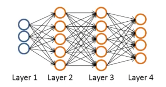
Neural Networks Representation

Logistic regression cannot form more complex hypotheses as it is only a linear classier. (You could add more features such as polynomial features to logistic regression, but that can be very expensive to train.)

The neural network will be able to represent complex models that form non-linear hypotheses.

Non-linear hypotheses

非线性回归在特征数过多时，特别是为了充分拟合数据，需要对特征进行组合（参考上章feature mappint)，将会产生更多的特征。

比如50x50的灰度图片，有2500的像素，即2500个特征值，如果需要两两组合(Quadratic features)，则有 $\binom{2}{2500} = \frac{2500\times2499}{2} \approx 3\times10^6$ 约300万个特征，如果三三组合，四四组合，百百组合呢？

Neurons and the grain

pass

Model representation

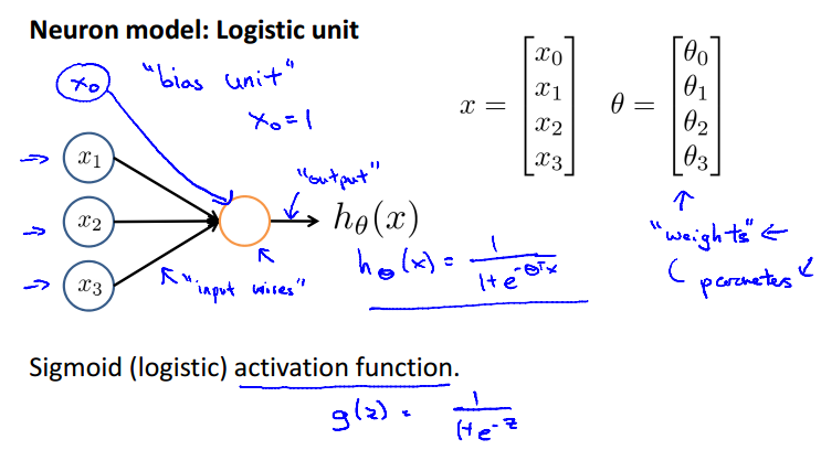神经元（Neuron）是大脑中的细胞。它的input wires是树突（Dendrite），output wires是轴突（Axon）。

in neural network:
$a_i^{(j)}$ = "activation" of unit i in layer j
$\Theta^{(j)}$ = matrix of weights controlling function mapping from layerj to layer j+1

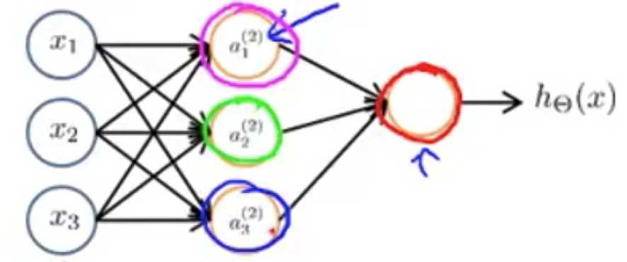
对于有一个hidden layer的神经网络： $\begin{aligned} a_1^{(2)} &= g(\Theta_{10}^{(1)}x_0+\Theta_{11}^{(1)}x_1+\Theta_{12}^{(1)}x_2+\Theta_{13}^{(1)}x_3) \\ a_2^{(2)} &= g(\Theta_{20}^{(1)}x_0+\Theta_{21}^{(1)}x_1+\Theta_{22}^{(1)}x_2+\Theta_{23}^{(1)}x_3) \\ a_3^{(2)} &= g(\Theta_{30}^{(1)}x_0+\Theta_{31}^{(1)}x_1+\Theta_{32}^{(1)}x_2+\Theta_{33}^{(1)}x_3) \\ h_\Theta(x) &= a_1{(3)} \\ &= g(\Theta_{10}^{(2)}a_0^{(2)}+\Theta_{11}^{(2)}a_1^{(2)}+\Theta_{12}^{(2)}a_2^{(2)}+\Theta_{13}^{(2)}a_3^{(2)}) \end{aligned}$

If layer 1 has 2 input nodes and layer 2 has 4 activation nodes. Dimension of $\Theta^{(1)}$ is going to be 4×3 where $s_j = 2$ and $s_{j+1} = 4$ , so $s_{j+1} \times (s_j + 1) = 4 \times 3$

Forward propagation: Vectorized implementation

上面的等式其实已经很明确地表现出了矩阵的形态，我们再令： $\Theta^{(i)}_jx_k = z^{(i)}_j$ $x = \begin{bmatrix}x_0\\x_1\\x_2\\x_3\end{bmatrix} \quad \quad z^{(2)} = \begin{bmatrix}z^{(2)}_1\\z^{(2)}_2\\z^{(2)}_3\\z^{(2)}_4\end{bmatrix}$

$z^{(2)} = \Theta^{(1)}x \quad (\rm{for\ uniform,\ set}\ x = a^{(1)}) \to z^{(2)} = \Theta^{(1)}a^{(1)}$ $a^{(2)} = g(z^{(2)})$

Add $a^{(2)}_0 = 1 \to$ $z^{(3)} = \Theta^{(2)}a^{(2)}$ $h_\Theta(x) = a^{(3)} = g(z^{(3)})$

梳理一下： $\begin{array}{|l|} \hline\\ \tt generalize: \\ \\ \begin{aligned} z^{(j)} &=\Theta^{(j−1)}a^{(j−1)} \\ a^{(j)} &= g(z^{(j)}) \\ z^{(j+1)} &= \Theta^{(j)}a^{(j)} \\ h_\Theta(x) &= a^{(j+1)} \\ &= g(z^{(j+1)})\\ \end{aligned} \\ \hline \end{array}$

Examples and Intuitions

假设 $x_1, x_2 \in {0 ,1}$ ，我们如何用神经网络来模拟 $x_1$ And $x_2$ ？

其实就是找出三个参数，让 $\theta_0 + \theta_1x_1 + \theta_2x_2$ 在不同的 $x_1, x_2$ 组合里分别得到预期的值，比如我们这里找到了[-30, 20, 20]，代入算式，以及回忆Sigmoid函数，求证：

$x_1$	$x_2$	exp	$y$
1	1	g(10)	1
0	0	g(-30)	0
1	0	g(-10)	0
0	1	g(-10)	0

see? exactly A&B

等于用四个训练样本来训练出合适的参数

试试自己求别的逻辑运算符？

现在我们要求 $x_1$ XNOR $x_2$ ，这是 $x_1$ XOR $x_2$ 的补集，对于XOR，只有在两者不同时为真时才为真，那么XNOR，显然为真时就是两者同时为0，或两者同时为1了。

由上一句话，我们是否可以得到三个逻辑运算符？

两者同时为0 即（not a) AND (not b)
两者同时为1 即（not a) OR (not b)
上述两者任意满足一个即可，1 OR 2

我们则可以把前两者输出到隐层，只专注一个判断，在Output layer才组合1和2
同时，隐层我们只关心全真，和全假，这两种情况，因此只需要两个节点，最后，不断的训练中，总能试到如下图的参数，从而产生了正确的输出，这里模型就算训练完毕了。

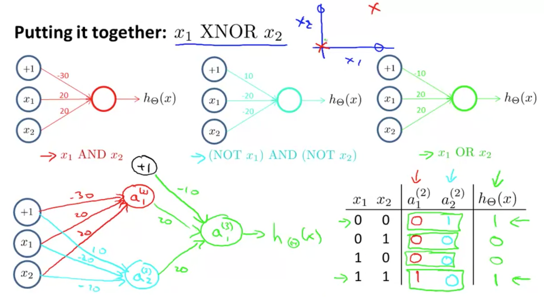
结论1:

我们得到了一个拆分特征，然后用新的特征去得到输出的例子。

结论2:

但如果写成代码，我们只会看写了三层，但不知道隐层输出了什么，因为代码并没有让第一层去找“全真，全假”，你能看到的就是权重相加，正向传播，然后反向传播。

结论3:

这里有一个很重要的点，即分层做了什么事，只是一个期望，并不是用代码去引导得来的。也就是说，如果得到的模型，其实它的各隐层其实是输出了别的特征与权重的组合，我们也不知道，以及，避免不了！

结论4:

也就是说，在编程的时候，我们明确知道需要一个什么样的模型，但不是去“指导”这个模型的每一层去做什么事，只能在梯度下降中（不然就是纯盲猜中）期望得到符合这个模型的参数。可能我们唯一能做的，就是根据我们的建模，去设置相应个数的隐层层数，每一个隐层的节点个数，以期最终训练出的模型是符合我们期待而不是别的模型的。

以上是神经网络能做复杂的事的最直观解释以及最完整例子了（你真的训练出了一个有实际意义的模型）。

Multi-class classification

比如一个识别交通工具的训练，首先，就是要把 $y \in \{1,2,3,4\}$ 改为 $y^{(i)}\ one\ of \begin{bmatrix} 1\\0\\0\\0\end{bmatrix}, \begin{bmatrix}0\\1\\0\\0\end{bmatrix},\cdots$ 有了前面的课程，想必也知道这是为了对应每一次output其实都会有4个输出，但只有一个是“可能性最高”的这样的形状（One-vs-rest），在编程实践中，也会把训练的对照结果提前变成矢量。

Neural Networks: Learning

Cost function

in Binary classification, y = 0 or 1, has 1 output unit, and $h_\theta(x) \in R^1$

in Multi-class classification, suppose we have k classes, the $h_\theta(x) \in R^k$ e.g. k = 4 $\begin{bmatrix}1\\0\\0\\0\end{bmatrix}, \begin{bmatrix}0\\1\\0\\0\end{bmatrix}, \begin{bmatrix}0\\0\\1\\0\end{bmatrix}, \begin{bmatrix}0\\0\\0\\1\end{bmatrix}$

$k\ge3$ , because if k==2, it can be a Binary classification

some symbols:

L: total number of layers in the network
$S_l$ : number of units (not counting bias unit) in layer l
K: number of output units/classes

recall logistic regression:

J(\theta) =-\frac{1}{m}\left[\sum_{i=1}^m{y^{(i)} \log(h_{\theta}(x^{(i)}))+(1-y^{(i)}) \log(1-h_{\theta}(x^{(i)}))}\right] +\frac{\lambda}{2m}\sum_{j=1}^n{\theta_j^2}

in Neural Network:

h_\Theta(x) \in R^K \quad (h_\Theta(x))_i = i^{th}\ \rm output

\begin{aligned} J(\Theta) = & -\frac{1}{m}\left[\sum_{i=1}^m\sum_{k=1}^K{y^{(i)}_k \log((h_{\Theta}(x^{(i)}))_k)+(1-y^{(i)}_k) \log(1-(h_{\Theta}(x^{(i)}))_k)}\right] \\ +&\frac{\lambda}{2m}\sum_{L=1}^{L-1}\sum_{i=1}^{S_l}\sum_{j=1}^{S_{l+1}}{(\Theta_{ij}^{(l)})^2} \end{aligned}

Note:

the double sum simply adds up the logistic regression costs calculated for each cell in the output layer
the triple sum simply adds up the squares of all the individual Θs in the entire network.
the i in the triple sum does not refer to training example i

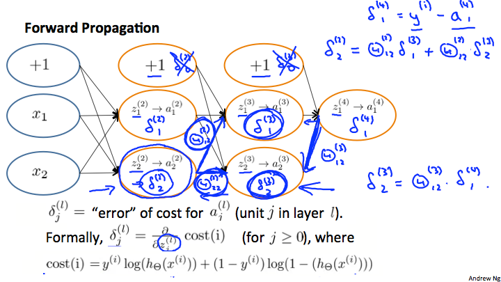
Back propagation algorithm(BP)

In order to use either gradient descent or one of the advance optimization algorithms, we need code to compute:

$J(\Theta)$
$\frac{\partial}{\partial\Theta_{ij}^{(l)}}J(\Theta)$

Intuition: $\delta_j^{(l)}$ = error of node j in layer l For each output unit (layer L=4) $\begin{aligned} \delta_j^{(4)} &= a_j^{(4)} - y_j \\ &=(h_\Theta(x))_j - y_j \\ &\underrightarrow{\,\ vectorization\ \,} \\ \delta^{(4)} &= a^{(4)} - y \\ \delta^{(3)} &= (\Theta^{(3)})^T\delta^{(4)}.*g'(z^{(3)}) \\ \delta^{(2)} &= (\Theta^{(2)})^T\delta^{(3)}.*g'(z^{(2)}) \end{aligned}$

注：

第L层output layer写成a-y是逻辑回归的cost function的导数的推导后的结果

所以其实它的公式跟其它隐层都是一样的，即上层的导数 * 本层激活函数的导数

如果g是sigmoid，那么 $g'(z^{(3)}) = a^{(3)} .* (1 - a^{(3)})$

back propagation指的就是这个 $\delta$ 由后向前传播的过程。

$\frac{\partial}{\partial\Theta_{ij}^{(l)}}J(\Theta) = a_j^{(l)}\delta_j^{(l+1)}$ ignoring $\lambda$ if $\lambda = 0$ （无证明步骤）

完整过程，for training set: $\{(x_{(1)}, y_{(1)}),(x_{(2)}, y_{(2)}),\dots,(x_{(m)}, y_{(m)})\}$

set $\Delta_{ij}^{(l)} = 0$ (for all l, i, j)

For i = 1 to m:

Set $a^{(1)} := x^{(i)}$ (hence you end up having a matrix full of zeros)
perform forward propagation to compute $a^{(l)}$ for l = 2, 3, ..., L
Using $y^{(i)}$ , compute $\delta^{(L)} = a^{(L)} - y^{(i)}$
Compute $\delta^{(L-1)}, \delta^{(L-2)},\dots,\delta^{(2)} \quad \red{\cancel{\delta^{(1)}}}$ using: $\delta^{(l)} = (\Theta^{(l)})^T\delta^{(l+1)} .* a^{(l)} .* (1 - a^{(l)})$
$\Delta_{ij}^{(l)} := \Delta_{ij}^{(l)} + a_j^{(l)}\delta_i^{(l+1)} \Rightarrow \Delta^{(l)} := \Delta^{(l)} + \delta^{(l+1)}(a^{(l)})^T$

最后： $\frac{\partial}{\partial\Theta_{ij}^{(l)}}J(\Theta) = \begin{cases} D_{ij}^{(l)} := \frac{1}{m}\Delta_{ij}^{(l)} &if\;\ j = 0 \\[2ex] D_{ij}^{(l)} := \frac{1}{m}\Delta_{ij}^{(l)} +\frac{\lambda}{m}\Theta_{ij}^{(l)} \quad &if\;\ j\ne 0 \end{cases}$

记住， $\delta_j^{(l)}$ is the error of cost for $a_j^{(l)}$ ，即 $\frac{\partial}{\partial z_j^{(l)}}cost(i)$

how to calculate $\delta$ :

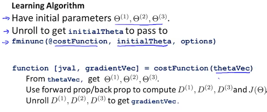
Uniforming parameters

要使用fminunc()，我们要把所有参数拍平送进去：

thetaVector = [ Theta1(:); Theta2(:); Theta3(:); ]
deltaVector = [ D1(:); D2(:); D3(:) ]

记住(:)是取出所有元素，并竖向排列

对于10x11, 10x11, 1x11的三个theta，在拍平后我们要还原的话：

Theta1 = reshape(thetaVector(1:110),10,11)
Theta2 = reshape(thetaVector(111:220),10,11)
Theta3 = reshape(thetaVector(221:231),1,11)

所以， octavea或matlab的切片是包头包尾的

Gradient checking

因为BP是如此复杂又黑盒，你往往不知道自己在层层求导的过程中每一步到底是不是对的，因为我们引入了检查机制，用非常微小的y变动除以相应非常微小的x变动来模拟一个导数，一般取 $10^{-4}$ 。

\frac{\partial}{\partial\theta_j}J(\Theta) = \frac{J(\Theta_1,\dots,\Theta_{j-\epsilon},\dots,\Theta_n) - J(\Theta_1,\dots,\Theta_{j+\epsilon},\dots,\Theta_n)} {2\epsilon}

如上每一个参数都检查一次，如果结果相当近似，说明你的代码是有用的，在训练前一定要记得关掉Gradient checking.

epsilon = 1e-4;
for i = 1:n,
  thetaPlus = theta;
  thetaPlus(i) += epsilon;
  thetaMinus = theta;
  thetaMinus(i) -= epsilon;
  gradApprox(i) = (J(thetaPlus) - J(thetaMinus))/(2*epsilon)
end;

Random initialization

Initializing all theta weights to zero does not work with neural networks. When we backpropagate, all nodes will update to the same value repeatedly. Instead we initialize each $\Theta_{ij}^{(l)}$ to a random value in $[-\epsilon, \epsilon]$

put together

make sure:

number of input units (aka features)
number of output units (aka classes)
number of hidden layers and units per layer (defaults: 1 hidden layer)

Training a Neural Network

randomly initialize the weights
implement forward propagation to get $h_\Theta(x^i)$ for any $x^i$
implement the cost function
implement backward propagation to compute partial derivatives
use gradient checking to confirm that your BP works, then disable gradient checking
use gradient descent or a built-in optimazation function to minimize the cost function with the weights in theta.

Advice for applying machine learning

为了让精度更高，我们可能会盲目采取如下做法：

get more training examples
try smaller sets of features
try getting additional features
try adding polynomial features ( $x^2_1, x^2_2, x_1x_2, etc.$ )
try decreasing / increasing $\lambda$

最终，有效的test才能保证你进行最有效的改进：Machine Learning diagnostic

Evaluating a hypothesis

拿一部分训练数据出来做测试数据(70%, 30%)，最好先打乱。(Training Set, Test Set)

对于线性回归问题，将训练集的参数应用到测试集，直接计算出测试集的误差即可： $J_{test}\Theta = \frac{1}{2m_{test}}\sum_{i=1}^{m_{test}}(h_\Theta(x^{(i)}_{test} - y^{(i)}_{test} ))^2$ 对于逻辑回归，应用0/1 misclassification error(错分率) $err(h_\Theta(x), y) = \begin{cases} 1 & if\ h_\Theta(x) \ge 0.5\ and\ y=0 \\ & \quad or \\ & h_\Theta(x) \lt 0.5\ y=1 \\ 0 & otherwise \end{cases}$ $Test\ Error = \frac{1}{m_{test}}\sum^{m_{test}}_{i=1}err$